Learn when & how to correctly use the Google Sheet VLOOKUP function with many easy-to-understand examples. Learn once, use anywhere.
When & Why Do You Need to Use VLOOKUP?
Whenever you want to fetch just a part of rows or columns from a large table, you shall consider using VLOOKUP to save your time.
For example, you are a popular English teacher and you’ve got a large final exam table containing the name and scores of all of your 500 students.
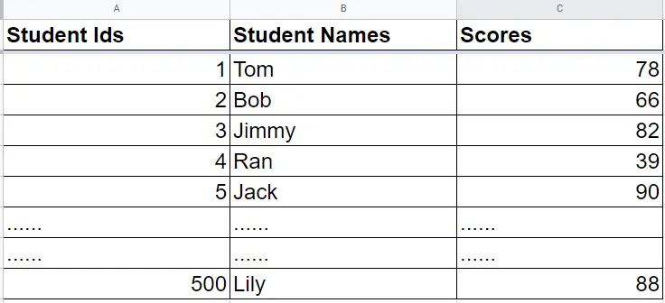
However, you’re eager to know the scores of your most concerned 10 students, in order to know if they have made big progress. But how can you quickly get their scores?
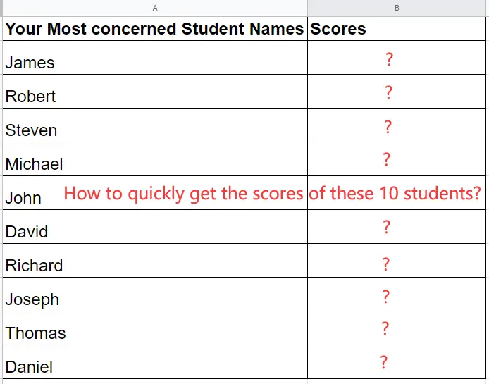
Search the students’ names from your large source table and find the scores one by one? What if you have 20, 30, or even 50 concerned students? That will be a lot of work. You need to learn the VLOOKUP formula to save your day.
Simply put, the VLOOKUP function can help you search for a value in one column, and return the corresponding value in another column.
Well, well, well, what does this mean? Don’t be afraid. I will give you a quick start example so that you can easily get started. Let’s go right now.
A Quick Start Example
To simplify everything, I have prepared an example products sheet, containing only 2 products’ names and prices:

Feel free to make a copy of this example sheet so that you can do the same exercise in this tutorial.
Now if you want to get the price of the iPhone, you can write down the following formula into any blank cells except columns G and H:
=VLOOKUP(“iPhone”, G:H, 2, FALSE)

Please note that you don’t need to use a formula to get the price in the real life. This is just an example.
Now, try to change the formula to
=VLOOKUP(“Galaxy”, G:H, 2, FALSE)
Can you get the correct price of $1,248?
You may notice that the VLOOKUP formula can help you search any product name in column G, and return its price in column H.
Don’t worry if now you can not understand why G:H, why 2, or why FALSE. I’m going to explain them one by one in the next chapter – the 4 parameters of the VLOOKUP function.
Detailed Explanation of the 4 Parameters of VLOOKUP
If you want the VLOOKUP function to work correctly, you need to explicitly specify 4 things:
1. The value to be searched for.
2. The range to consider for the search.
3. The column index of the value to be returned.
4. Whether using the fuzzy matching or not.
Let me first explain the 2nd parameter, because it is the most important one.
The 2nd Parameter – Specify the Search Area
Actually, the VLOOKUP function only searches for a value in the first column of a specified range. Yes, the first column of a range.
So, the example formula =VLOOKUP(“iPhone”, G:H, 2, FALSE) in the quick start section was to state that, please search for “iPhone” in the first column of range G:H. Of course, the first column of G:H is G.

Whenever you use VLOOKUP, make sure the range starts with the column that you want to search for a value.
And you should ensure that the range contains the column that holds the return value. Why? This brings us to the 3rd parameter.
The 3rd Parameter – The Column Index in the Range That Holds the Return Value
Remember the purpose of using VLOOKUP? Get the corresponding value of the searched value. What you want to get is the related value, not the searched value.
And to get the related value, you need to specify the index of the column based on the range. The index of column H is 2 in the range G:H.

What if we change the example table structure by inserting 1 color column? If we still want to get the price of the iPhone, what should the formula be?

It should be =VLOOKUP(“iPhone”, G:I, 3, FALSE)
To search “iPhone”, the range should start with column G. And to get the price, the range should contain column I. Finally, the index of column I is 3 in the range G:I.

The 4th Parameter – Using Fuzzy Matching or Not
In most cases, it is highly recommended that you set the 4th parameter to FALSE to avoid getting an incorrect result. If you want to know more details, keep reading.
When to Use Fuzzy Matching and How It Works
The 4th parameter of VLOOKUP is to indicate whether to use fuzzy matching. When it is set to TRUE, Google Sheets will search for the value less than or equal to the search key. When set to FALSE, only exact matching will be used. The default value of this parameter is TRUE.
You may wonder why we need fuzzy matching, as we just want to look up the exact value. Let’s look at another example. Suppose you are a math teacher, and you want to get the grade of your students according to their final exam scores.
The score-grade table looks like this:
| Score | Grade |
| 0 | D |
| 60 | C |
| 80 | B |
| 90 | A |
Grade D is for 0-60, C for 60-80, B for 80-90, and A for 90+.
And the final exam table looks like this:
| Name | Score | Grade |
| Tom | 46 | ? |
| Lily | 88 | ? |
| Bob | 99 | ? |
How can you get the grade of each student based on the score? Can you use the exact matching mode in this example? Obviously not. You can not find the exact scores 46, 88, and 99 in the score-grade table. But it is reasonable to search for a value less than 46, 88, or 99. This is the perfect case to use fuzzy matching.
If we want to get the grade for Tom’s final exam, our formula should be:
=VLOOKUP(46, G:H, 2, TRUE)
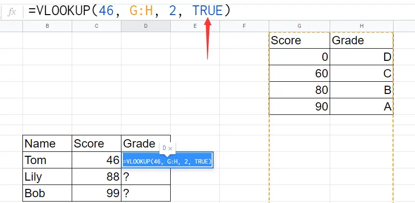
What does this formula mean? We’re telling VLOOKUP that please find a value less than or equal to 46 in column G. If you can find such a value, return its grade in column H.
As we already said that if a score is less than 60, the grade should be D. Tom got 46, which is less than 60. And in column G, only 0 is the nearest value less than 46. That’s why we can get the correct grade.
For Lily, the nearest value less than 88 in column G is 80, so the formula to get Lily’s grade is =VLOOKUP(80, G:H, 2, TRUE).
I think it’s easy now for you to finish the formula to fetch Bob’s grade. Go ahead to write down the formula yourself and understand once more how fuzzy matching works.
2 Things You Need to Notice When Using Fuzzy Matching
After you totally understand the difference between exact matching and fuzzy matching, let’s talk about what you should notice when dealing with fuzzy matching, which can help you avoid getting the wrong result.
Do Not Use Fuzzy Matching to Search Strings
It doesn’t make any sense to search a string less than another string. You may get an incorrect result if you do this, even though we can compare strings according to their ASCII code from the left one by one. However, this will make things complicated, so just use this when you want to search for a number that is less than or equal to another number.
Make Sure the First Column of the Range Is in Ascending Order
You will get the wrong result if the search column is not in ascending order. Try to change the score-grade table as follow:
| Score | Grade |
| 0 | D |
| 90 | A |
| 80 | B |
| 60 | C |
You will get the wrong grades for Lily and Bob.
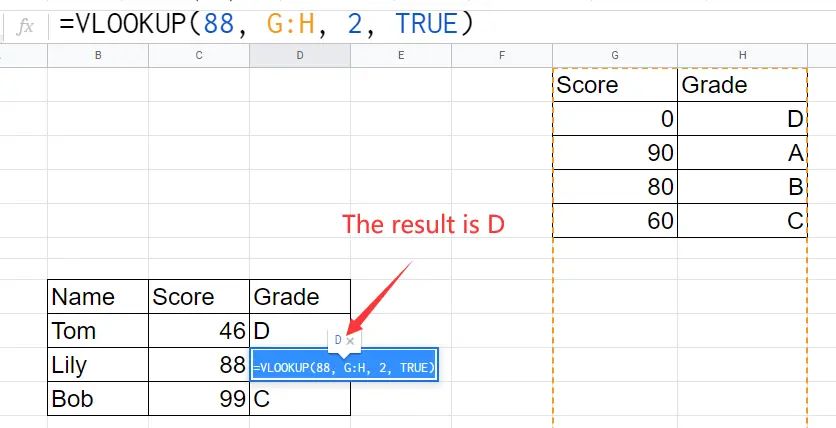
I will not go deeper into this. Just keep in mind that if you want to find a value that is less than another value, a sorted column in ascending order will help VLOOKUP find that value correctly and quickly. Do not fool Google Sheets if you want to work with it.
The 1st Parameter – What You Want to Find
The first parameter of the VLOOKUP function is much easier to understand, but I’d like to include more details about this parameter, which can help you work more efficiently and stay away from some mistakes.
The First Parameter Is Case Insensitive
In our quick start example, we fetch the price of “iPhone” by formula =VLOOKUP(“iPhone”, G:H, 2, FALSE). However, if we use =VLOOKUP(“iphone”, G:H, 2, FALSE) we can still get the right price.
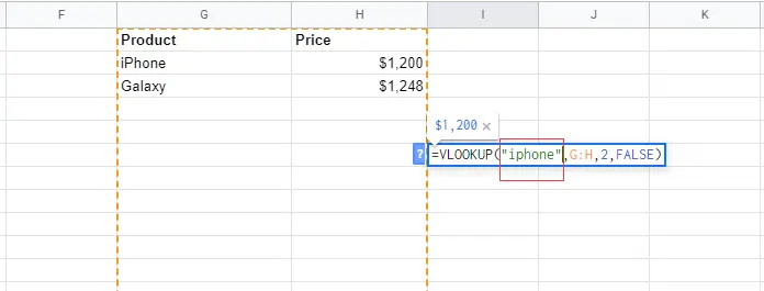
When we use the VLOOKUP function to search for a string value, Google Sheets will ignore the case, which will save us a lot of time and energy as we don’t need to consider the case. But sometimes, you might get the wrong result because of this default behavior of the VLOOKUP formula.
If we add one more row in our example table:
| Product | Price |
| iphone | $1,000 |
| iPhone | $1,200 |
| Galaxy | $1,248 |
What the result of =VLOOKUP(“iPhone”,G:H,2,FALSE) will be? $1,000 or $1,200? Unfortunately, the result is $1,000.

We explicitly indicated that we want to search for “iPhone”, not “iphone”. Why did we still get $1,000, not $1,200?
Without considering the case, “Iphone”, “iPhone”, “IPHONE”, even “iPhONE” are the same word. Ignoring the case, the VLOOKUP function will stop matching when it finds the first same value.
I strongly recommend that you check your source table and make sure the column to be searched only contains unique values. Otherwise, you may get an incorrect result.
The First Parameter Can Be a Reference to a Cell
In the previous examples, we explicitly tell VLOOKUP which value we want to search for. However, it can also be a reference to another cell just like any other formula in Google Sheets.
Again, let’s use the example table in the quick start section. Besides using the formula =VLOOKUP(“iPhone”, G:H, 2, FALSE), we can also get the right result by using =VLOOKUP(G2, G:H, 2, FALSE), as the value of cell G2 is “iPhone”.
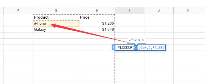
Using references to other cells is more convenient if you have a lot of values to be searched for. What’s more, you don’t need to modify the formula if the value to be searched for needs to be updated.
Another benefit of using references is that when you drop down your first formula, Google Sheets will automatically fill the references. Open our example sheets and go to the sheet “Use Cell Reference in the first parameter”. Let’s find the scores of the most concerned 10 students without manually writing down 10 formulas.
Put the following formula into cell F6:
=VLOOKUP(E6,A:B,2,FALSE)
Press the left button of your mouse and pull down from the right bottom corner of F6, until F15.
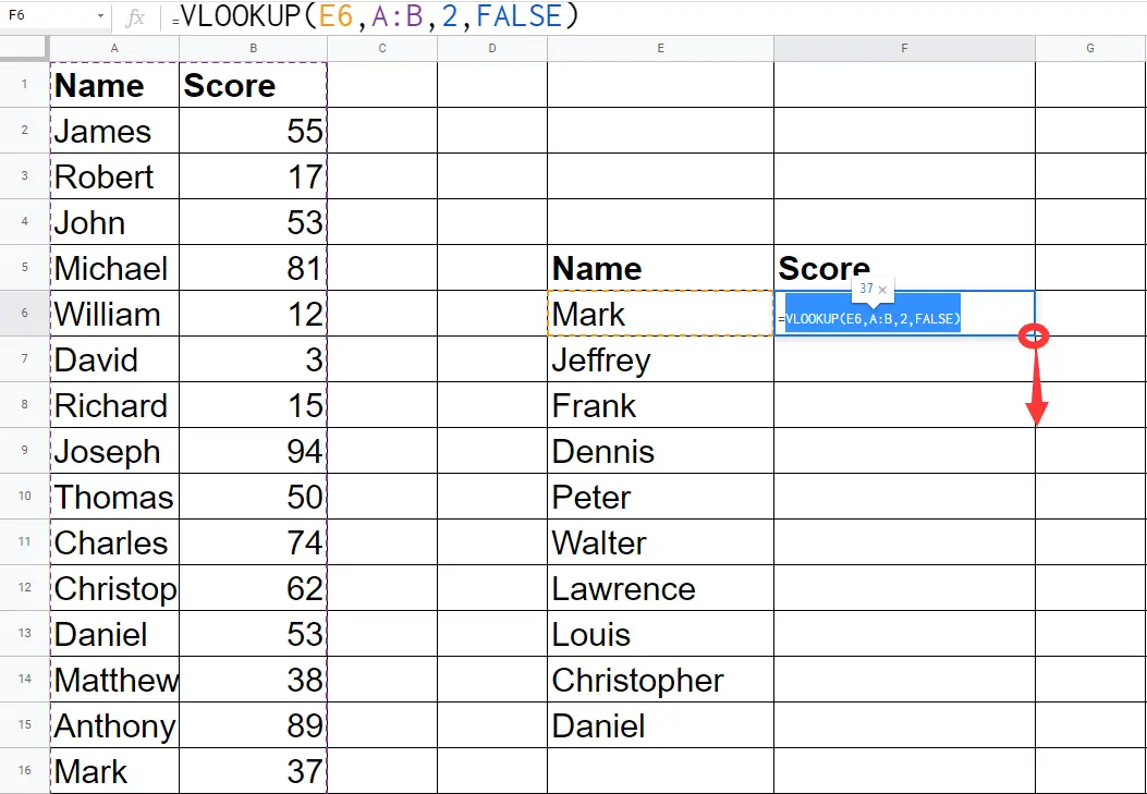
Google Sheets will automatically fill all formulas from F7 to F15. This will save you a lot of time when you have a lot of values that need to be searched.
Wildcards Can Be Used
The last point about the first 1 parameter is that you can use 2 wildcards (the question mark ? and the asterisk *) to find matches. Just like the fuzzy matching, you will not need to use wildcards in most cases. But I will give you a very simple example for a complete guide.
The question mark stands in for a single character while the asterisk for any series of characters. For instance, iPhone? can match iPhone6, and iPhone8, but can not match iPhone12. However, iPhone* can match iPhone6, iPhone8, even iPhone12.
If you need to match an actual question mark or asterisk, add a tilde (~) before the character and add an extra tilde if you’re looking for something with an actual tilde in it.
How to Handle the VLOOKUP #N/A Error
We already know that the first and second parameters of VLOOKUP indicate Google Sheets to find the specific value in the first column of a range. But what if the column doesn’t contain the value?
Again, open our example spreadsheet and visit the Error Handling sheet, where we want to get the score for Jason but there is no Jason’s record in our source data.
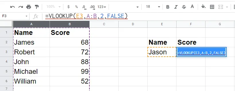
What will we get? A #N/A error value.
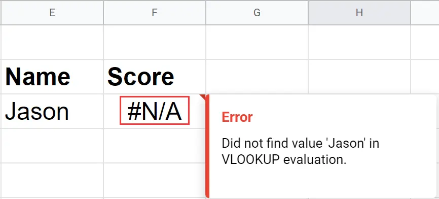
The VLOOKUP function will return the #N/A error when the specific value can not be found in that column. If we want to remove the #N/A error or replace #n/a with blank we can combine the IFERROR and VLOOKUP function in Google Sheets.
The 2nd parameter of the IFERROR formula gives you the right to decide what to return when an error occurs. If you omit this argument, it will return nothing.
Now let’s use the IFEROR function to wrap our VLOOKUP formula:
=IFERROR(VLOOKUP(E3,A:B,2,FALSE))

The VLOOKUP #N/A error value will disappear. Since we left the 2nd parameter of IFERROR blank, nothing will be displayed in cell F3.
Congratulations! You have learned all of the basic usages of VLOOKUP. You are able to write a correct VLOOKUP formula now whenever you want to search for a value in one column and return the corresponding value in another column.
But if you are a heavy user of Google Sheets and want to know more advanced usage of this function, you may not want to miss out on the following chapters.
How to Use Google Sheets VLOOKUP From Another Sheet
You may notice that the values we want to search for and the source data are in the same sheet across all of the above examples. However, we usually have to work with multiple worksheets.
How to do VLOOKUP in Google Sheets when the search values and the source data are not in the same sheet, even when they are not in the same workbook? Let’s talk about them one by one.
Use VLOOKUP From a Different Sheet in the Same Workbook
Let’s firstly talk about the former case – in the same workbook but on a different sheet. Now open our example sheets and go to the “Query from Error Handling” sheet where we need to find Robert’s score from the “Error Handling” sheet.
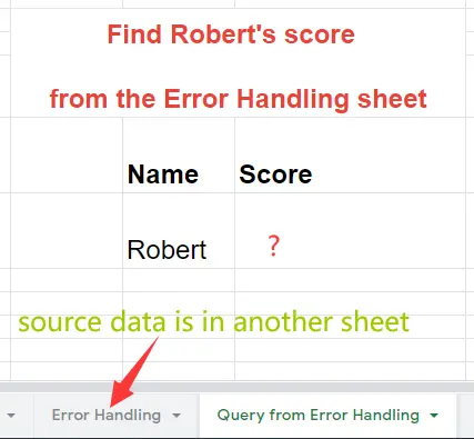
What should the VLOOKUP formula be? Fortunately, you don’t need to worry about this because Google Sheets has already automatically solved this problem for us.
When you are going to write the 2nd argument, just click the “Error Handling” sheet.
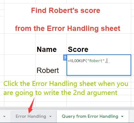
Then just select Range A:B. Google Sheets will automatically add the sheet name before the range, so you will see the range becomes ‘Error Handling’!A:B.
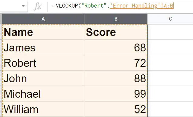
Actually, you are now writing the formula in the “Error Handling” sheet. So just add a comma and finish the left arguments.
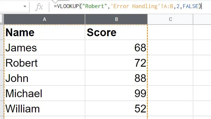
Now press enter on your keyboard, and you will be back to the “Query from Error Handling” sheet with the correct result showing.

Obviously, you can manually add the sheet name plus the exclamation mark – ‘Error Handling’! before the range. This way, you don’t need to jump between different sheets. Manually adding the prefix or not depends on if the sheet name is easy to type. You can decide it yourself when you need to use google sheets VLOOKUP from another tab in the same spreadsheet.
Use VLOOKUP From Another Workbook in Google Sheets
Things will become complicated if you want to match a value from another sheet in a different spreadsheet. Unlike the last case, there is no prefix exclusively for another workbook.
I have prepared the source data from another workbook. Kindly make a copy of our spreadsheet according to the following URL:
https://docs.google.com/spreadsheets/d/1SRjcHk_Z4He-SQ57fTLKUbw7axqdKoX-VwYqp-YMniY/edit?usp=sharing
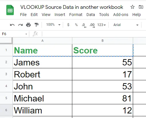
Now visit the “Query from another workbook” sheet in our example spreadsheet. How can we get Andrew’s score?
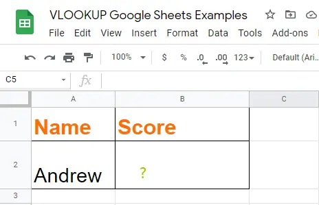
The only solution for doing VLOOKUP from another workbook in Google Sheets is to first import the source data to the workbook where you need to use VLOOKUP. Then you can use the VLOOKUP function as usual in the same workbook. And to import data from another spreadsheet, you need the help of the IMPORTRANGE function.
If you want to know more details, check our IMPORTRANGE Google Sheets Tutorial. The only thing to remind is that make sure you can access the target spreadsheet if you need to import data from another spreadsheet.
Here I will directly give the final formula to import source data from our example spreadsheet:
=IMPORTRANGE("https://docs.google.com/spreadsheets/d/1SRjcHk_Z4He-SQ57fTLKUbw7axqdKoX-VwYqp-YMniY/edit?usp=sharing", "Sheet1!A:B")Now that you have imported the data, I think you are able to find Andrew’s score, right? Try to finish the formula as soon as you can and move to the next part.
ARRAYFORMULA With VLOOKUP Google Sheets
Think about this case – you need to fetch 500 students’ scores from a large source table containing 5, 000 records. How can you quickly achieve this?

If you just write the first VLOOKUP formula and pull it down until Google Sheets fills all of the 500 VLOOKUP functions, that will be a lot of time. And I’m sure your right hand will not feel very well. Can we just write one formula to fetch 500, or even 500,000 results without pulling down a formula? Yes, you can save your time by using ARRAYFORMULA and VLOOKUP together in Google Sheets.
For those who do not know, the ARRAYFORMULA can return a bunch of results, not just a single result like other formulas. If you want to know more details of this function, check our ARRAYFORMULA tutorial.
Now open our example sheet and go to the arrayformula sheet, and let’s just write just one formula in F2 to get 20 students’ scores.
One formula to get all scores? How? Let’s finish it with 3 steps.
Firstly, let’s finish the formula to get John’s score. It should be =VLOOKUP(E2,A:B,2,FALSE). Take a good look at the 1st argument of this formula: E2. We only tell Google Sheets to query E2. Why not tell Google Sheets to help us query E2:E21?
Now change our formula to =VLOOKUP(E2:E21,A:B,2,FALSE). Of course, this formula will not work because VLOOKUP can only query one value once a time. But if we wrap it with ARRAYFORMULA, that is to say, =ARRAYFORMULA(VLOOKUP(E2:E21,A:B,2,FALSE)), we will get all scores immediately.
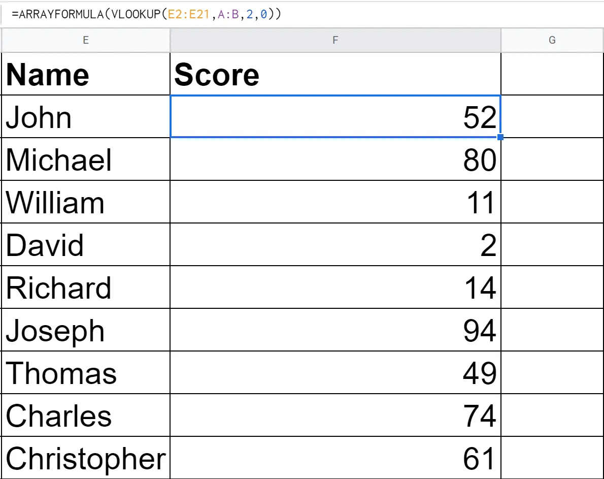
Yes, we made it! Use just one formula to get all students’ scores. Keep in mind that when using ARRAYFORMULA with VLOOKUP to query a lot of values, the 1st argument of VLOOKUP should be a range, not a single value.
Use VLOOKUP to Fetch Multiple Columns In Google Sheets
In all of the examples above, we only fetch one column of a range. However, we are able to fetch multiple columns at the same time when using VLOOKUP.
Now kindly open the “Multiple Columns” sheet in our example sheets, and let’s use one formula to fetch John’s age and score at the same time.
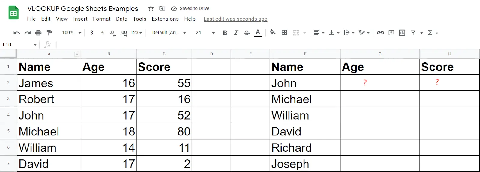
When you want to fetch multiple values (columns) when using VLOOKUP, you need to put the indexes of the columns within curly braces when specifying the 3rd argument of VLOOKUP. In our example, it should be {2,3}.
Once again, because VLOOKUP can only return a single result by default, if we need to return multiple values, we need to use ARRAYFORMULA. Therefore, the formula to fetch both John’s age and score should be =ARRAYFORMULA(VLOOKUP(F2, A:C, {2,3}, 0))
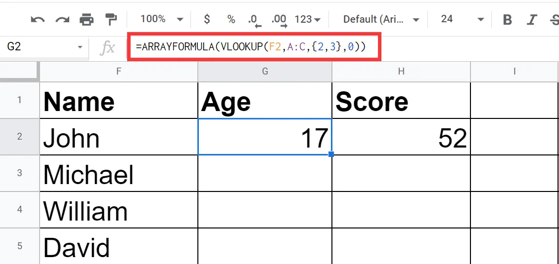
Now let’s take one step further – use one formula to fetch all 20 students’ ages and scores at the same time. Can you finish the formula yourself?
The correct answer is =ARRAYFORMULA(VLOOKUP(F2:F21,A:C,{2,3},0)).
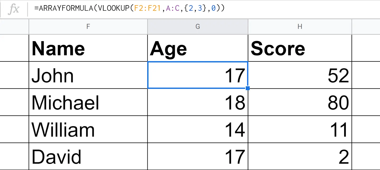
We want to query 20 students at the same time, so the 1st argument is F2:F21. We want to return both ages and scores, so the 3rd argument is {2,3}. And because we return multiple values, we need to use ARRAYFORMULA. Is everything clear now?
=ARRAYFORMULA(VLOOKUP(F2:F21, A:C, {2,3}, 0)) is the most complicated formula we have met in this guide. If you can totally understand it, you will have no problem handling any VLOOKUP cases.
And this is the perfect place where we shall put an end to this tutorial.